An increasing number of modern antivirus solutions rely on machine learning (ML) techniques to protect users from malware. While ML-based approaches, like FireEye Endpoint Security’s MalwareGuard capability, have done a great job at detecting new threats, they also come with substantial development costs. Creating and curating a large set of useful features takes significant amounts of time and expertise from malware analysts and data scientists (note that in this context a feature refers to a property or characteristic of the executable that can be used to distinguish between goodware and malware). In recent years, however, deep learning approaches have shown impressive results in automatically learning feature representations for complex problem domains, like images, speech, and text. Can we take advantage of these advances in deep learning to automatically learn how to detect malware without costly feature engineering?

As it turns out, deep learning architectures, and in particular convolutional neural networks (CNNs), can do a good job of detecting malware simply by looking at the raw bytes of Windows Portable Executable (PE) files. Over the last two years, FireEye has been experimenting with deep learning architectures for malware classification, as well as methods to evade them. Our experiments have demonstrated surprising levels of accuracy that are competitive with traditional ML-based solutions, while avoiding the costs of manual feature engineering. Since the initial presentation of our findings, other researchers have published similarly impressive results, with accuracy upwards of 96%.

Since these deep learning models are only looking at the raw bytes without any additional structural, semantic, or syntactic context, how can they possibly be learning what separates goodware from malware? In this blog post, we answer this question by analyzing FireEye’s deep learning-based malware classifier.

Background

Before we dive into our analysis, let’s first discuss what a CNN classifier is doing with Windows PE file bytes. Figure 1 shows the high-level operations performed by the classifier while “learning” from the raw executable data. We start with the raw byte representation of the executable, absent any structure that might exist (1). This raw byte sequence is embedded into a high-dimensional space where each byte is replaced with an n-dimensional vector of values (2). This embedding step allows the CNN to learn relationships among the discrete bytes by moving them within the n-dimensional embedding space. For example, if the bytes 0xe0 and 0xe2 are used interchangeably, then the CNN can move those two bytes closer together in the embedding space so that the cost of replacing one with the other is small. Next, we perform convolutions over the embedded byte sequence (3). As we do this across our entire training set, our convolutional filters begin to learn the characteristics of certain sequences that differentiate goodware from malware (4). In simpler terms, we slide a fixed-length window across the embedded byte sequence and the convolutional filters learn the important features from across those windows. Once we have scanned the entire sequence, we can then pool the convolutional activations to select the best features from each section of the sequence (i.e., those that maximally activated the filters) to pass along to the next level (5). In practice, the convolution and pooling operations are used repeatedly in a hierarchical fashion to aggregate many low-level features into a smaller number of high-level features that are more useful for classification. Finally, we use the aggregated features from our pooling as input to a fully-connected neural network, which classifies the PE file sample as either goodware or malware (6).

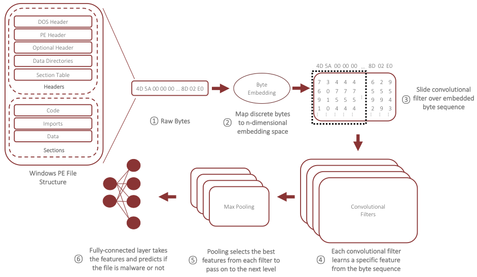
The specific deep learning architecture that we analyze here actually has five convolutional and max pooling layers arranged in a hierarchical fashion, which allows it to learn complex features by combining those discovered at lower levels of the hierarchy. To efficiently train such a deep neural network, we must restrict our input sequences to a fixed length – truncating any bytes beyond this length or using special padding symbols to fill out smaller files. For this analysis, we chose an input length of 100KB, though we have experimented with lengths upwards of 1MB. We trained our CNN model on more than 15 million Windows PE files, 80% of which were goodware and the remainder malware. When evaluated against a test set of nearly 9 million PE files observed in the wild from June to August 2018, the classifier achieves an accuracy of 95.1% and an F1 score of 0.96, which are on the higher end of scores reported by previous work.

In order to figure out what this classifier has learned about malware, we will examine each component of the architecture in turn. At each step, we use either a sample of 4,000 PE files taken from our training data to examine broad trends, or a smaller set of six artifacts from the NotPetya, WannaCry, and BadRabbit ransomware families to examine specific features.

Bytes in (Embedding) Space

The embedding space can encode interesting relationships that the classifier has learned about the individual bytes and determine whether certain bytes are treated differently than others because of their implied importance to the classifier’s decision. To tease out these relationships, we will use two tools: (1) a dimensionality reduction technique called multi-dimensional scaling (MDS) and (2) a density-based clustering method called HDBSCAN. The dimensionality reduction technique allows us to move from the high-dimensional embedding space to an approximation in two-dimensional space that we can easily visualize, while still retaining the overall structure and organization of the points. Meanwhile, the clustering technique allows us to identify dense groups of points, as well as outliers that have no nearby points. The underlying intuition being that outliers are treated as “special” by the model since there are no other points that can easily replace them without a significant change in upstream calculations, while dense clusters of points can be used interchangeably.

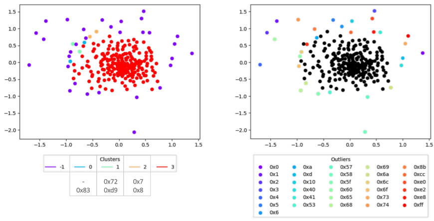
On the left side of Figure 2, we show the two-dimensional representation of our byte embedding space with each of the clusters labeled, along with an outlier cluster labeled as -1. As you can see, the vast majority of bytes fall into one large catch-all class (Cluster 3), while the remaining three clusters have just two bytes each. Though there are no obvious semantic relationships in these clusters, the bytes that were included are interesting in their own right – for instance, Cluster 0 includes our special padding byte that is only used when files are smaller than the fixed-length cutoff, and Cluster 1 includes the ASCII character ‘r.’

What is more fascinating, however, is the set of outliers that the clustering produced, which are shown in the right side of Figure 3.  Here, there are a number of intriguing trends that start to appear. For one, each of the bytes in the range 0x0 to 0x6 are present, and these bytes are often used in short forward jumps or when registers are used as instruction arguments (e.g., eax, ebx, etc.). Interestingly, 0x7 and 0x8 are grouped together in Cluster 2, which may indicate that they are used interchangeably in our training data even though 0x7 could also be interpreted as a register argument. Another clear trend is the presence of several ASCII characters in the set of outliers, including ‘\n’, ‘A’, ‘e’, ‘s’, and ‘t.’ Finally, we see several opcodes present, including the call instruction (0xe8), loop and loopne (0xe0, 0xe2), and a breakpoint instruction (0xcc).

Given these findings, we immediately get a sense of what the classifier might be looking for in low-level features: ASCII text and usage of specific types of instructions.

Deciphering Low-Level Features

The next step in our analysis is to examine the low-level features learned by the first layer of convolutional filters. In our architecture, we used 96 convolutional filters at this layer, each of which learns basic building-block features that will be combined across the succeeding layers to derive useful high-level features. When one of these filters sees a byte pattern that it has learned in the current convolution, it will produce a large activation value and we can use that value as a method for identifying the most interesting bytes for each filter. Of course, since we are examining the raw byte sequences, this will merely tell us which file offsets to look at, and we still need to bridge the gap between the raw byte interpretation of the data and something that a human can understand. To do so, we parse the file using PEFile and apply BinaryNinja’s disassembler to executable sections to make it easier to identify common patterns among the learned features for each filter.

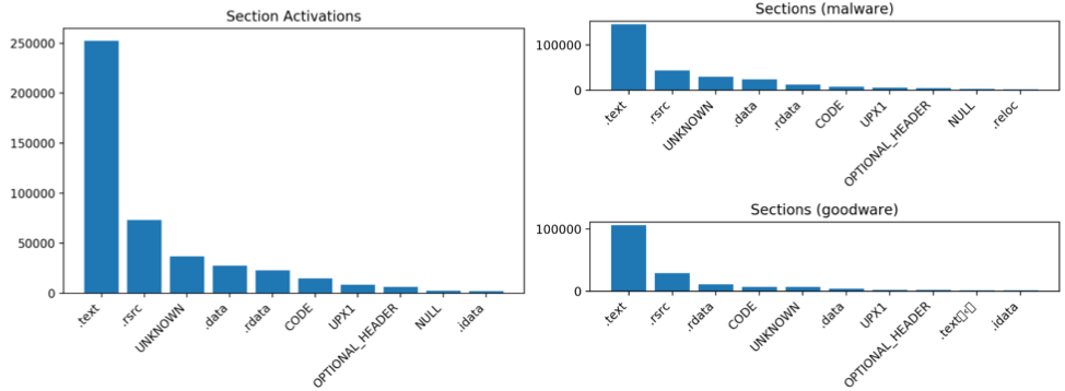
Since there are a large number of filters to examine, we can narrow our search by getting a broad sense of which filters have the strongest activations across our sample of 4,000 Windows PE files and where in those files those activations occur. In Figure 3, we show the locations of the 100 strongest activations across our 4,000-sample dataset. This shows a couple of interesting trends, some of which could be expected and others that are perhaps more surprising. For one, the majority of the activations at this level in our architecture occur in the ‘.text’ section, which typically contains executable code. When we compare the ‘.text’ section activations between malware and goodware subsets, there are significantly more activations for the malware set, meaning that even at this low level there appear to be certain filters that have keyed in on specific byte sequences primarily found in malware. Additionally, we see that the ‘UNKNOWN’ section– basically, any activation that occurs outside the valid bounds of the PE file – has many more activations in the malware group than in goodware. This makes some intuitive sense since many obfuscation and evasion techniques rely on placing data in non-standard locations (e.g., embedding PE files within one another).

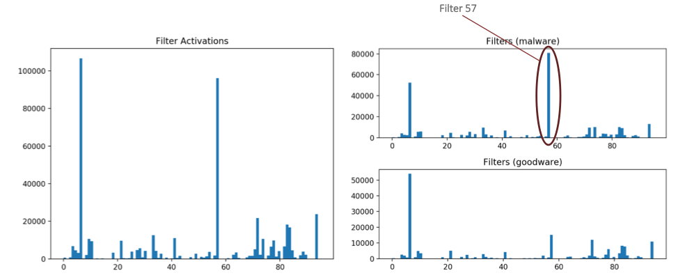
We can also examine the activation trends among the convolutional filters by plotting the top-100 activations for each filter across our 4,000 PE files, as shown in Figure 4. Here, we validate our intuition that some of these filters are overwhelmingly associated with features found in our malware samples. In this case, the activations for Filter 57 occur almost exclusively in the malware set, so that will be an important filter to look at later in our analysis. The other main takeaway from the distribution of filter activations is that the distribution is quite skewed, with only two filters handling the majority of activations at this level in our architecture. In fact, some filters are not activated at all on the set of 4,000 files we are analyzing.

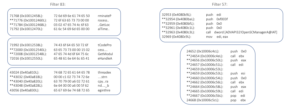
Now that we have identified the most interesting and active filters, we can disassemble the areas surrounding their activation locations and see if we can tease out some trends. In particular, we are going to look at Filters 83 and 57, both of which were important filters in our model based on activation value. The disassembly results for these filters across several of our ransomware artifacts is shown in Figure 5.

For Filter 83, the trend in activations becomes pretty clear when we look at the ASCII encoding of the bytes, which shows that the filter has learned to detect certain types of imports. If we look closer at the activations (denoted with a ‘*’), these always seem to include characters like ‘r’, ‘s’, ‘t’, and ‘e’, all of which were identified as outliers or found in their own unique clusters during our embedding analysis.  When we look at the disassembly of Filter 57’s activations, we see another clear pattern, where the filter activates on sequences containing multiple push instructions and a call instruction – essentially, identifying function calls with multiple parameters.

In some ways, we can look at Filters 83 and 57 as detecting two sides of the same overarching behavior, with Filter 83 detecting the imports and 57 detecting the potential use of those imports (i.e., by fingerprinting the number of parameters and usage). Due to the independent nature of convolutional filters, the relationships between the imports and their usage (e.g., which imports were used where) is lost, and that the classifier treats these as two completely independent features.

Aside from the import-related features described above, our analysis also identified some filters that keyed in on particular byte sequences found in functions containing exploit code, such as DoublePulsar or EternalBlue. For instance, Filter 94 activated on portions of the EternalRomance exploit code from the BadRabbit artifact we analyzed. Note that these low-level filters did not necessarily detect the specific exploit activity, but instead activate on byte sequences within the surrounding code in the same function.

These results indicate that the classifier has learned some very specific byte sequences related to ASCII text and instruction usage that relate to imports, function calls, and artifacts found within exploit code. This finding is surprising because in other machine learning domains, such as images, low-level filters often learn generic, reusable features across all classes.

Bird’s Eye View of End-to-End Features

While it seems that lower layers of our CNN classifier have learned particular byte sequences, the larger question is: does the depth and complexity of our classifier (i.e., the number of layers) help us extract more meaningful features as we move up the hierarchy? To answer this question, we have to examine the end-to-end relationships between the classifier’s decision and each of the input bytes. This allows us to directly evaluate each byte (or segment thereof) in the input sequence and see whether it pushed the classifier toward a decision of malware or goodware, and by how much. To accomplish this type of end-to-end analysis, we leverage the SHapley Additive exPlanations (SHAP) framework developed by Lundberg and Lee. In particular, we use the GradientSHAP method that combines a number of techniques to precisely identify the contributions of each input byte, with positive SHAP values indicating areas that can be considered to be malicious features and negative values for benign features.

After applying the GradientSHAP method to our ransomware dataset, we noticed that many of the most important end-to-end features were not directly related to the types of specific byte sequences that we discovered at lower layers of the classifier. Instead, many of the end-to-end features that we discovered mapped closely to features developed from manual feature engineering in our traditional ML models. As an example, the end-to-end analysis on our ransomware samples identified several malicious features in the checksum portion of the PE header, which is commonly used as a feature in traditional ML models. Other notable end-to-end features included the presence or absence of certain directory information related to certificates used to sign the PE files, anomalies in the section table that define the properties of the various sections of the PE file, and specific imports that are often used by malware (e.g., GetProcAddress and VirtualAlloc).

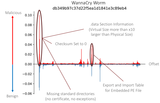
In Figure 6, we show the distribution of SHAP values across the file offsets for the worm artifact of the WannaCry ransomware family. Many of the most important malicious features found in this sample are focused in the PE header structures, including previously mentioned checksum and directory-related features. One particularly interesting observation from this sample, though, is that it contains another PE file embedded within it, and the CNN discovered two end-to-end features related to this. First, it identified an area of the section table that indicated the ‘.data’ section had a virtual size that was more than 10x larger than the stated physical size of the section. Second, it discovered maliciously-oriented imports and exports within the embedded PE file itself. Taken as a whole, these results show that the depth of our classifier appears to have helped it learn more abstract features and generalize beyond the specific byte sequences we observed in the activations at lower layers.

Summary

In this blog post, we dove into the inner workings of FireEye’s byte-based deep learning classifier in order to understand what it, and other deep learning classifiers like it, are learning about malware from its unstructured raw bytes. Through our analysis, we have gained insight into a number of important aspects of the classifier’s operation, weaknesses, and strengths:

• Import Features: Import-related features play a large role in classifying malware across all levels of the CNN architecture. We found evidence of ASCII-based import features in the embedding layer, low-level convolutional features, and end-to-end features.
• Low-Level Instruction Features: Several features discovered at the lower layers of our CNN classifier focused on sequences of instructions that capture specific behaviors, such as particular types of function calls or code surrounding certain types of exploits. In many cases, these features were primarily associated with malware, which runs counter to the typical use of CNNs in other domains, such as image classification, where low-level features capture generic aspects of the data (e.g., lines and simple shapes). Additionally, many of these low-level features did not appear in the most malicious end-to-end features.
• End-to-End Features: Perhaps the most interesting result of our analysis is that many of the most important maliciously-oriented end-to-end features closely map to common manually-derived features from traditional ML classifiers. Features like the presence or absence of certificates, obviously mangled checksums, and inconsistencies in the section table do not have clear analogs to the lower-level features we uncovered. Instead, it appears that the depth and complexity of our CNN classifier plays a key role in generalizing from specific byte sequences to meaningful and intuitive features.

It is clear that deep learning offers a promising path toward sustainable, cutting-edge malware classification. At the same time, significant improvements will be necessary to create a viable real-world solution that addresses the shortcomings discussed in this article. The most important next step will be improving the architecture to include more information about the structural, semantic, and syntactic context of the executable rather than treating it as an unstructured byte sequence. By adding this specialized domain knowledge directly into the deep learning architecture, we allow the classifier to focus on learning relevant features for each context, inferring relationships that would not be possible otherwise, and creating even more robust end-to-end features with better generalization properties.

The content of this blog post is based on research presented at the Conference on Applied Machine Learning for Information Security (CAMLIS) in Washington, DC on Oct. 12-13, 2018. Additional material, including slides and a video of the presentation, can be found on the conference website.

An extended version of the research presented in this blog post can be found in our peer-reviewed paper from the IEEE Deep Learning and Security workshop. A publicly-available version of the paper is also available.